


Shifting from Meters to Centimeters: Deep-Diving UWB Architecture for Precision RTLS
A Comprehensive Guide on Hardware Node Topologies, Signaling Mathematics, and Geometric Constraints in Next-Generation Asset Tracking
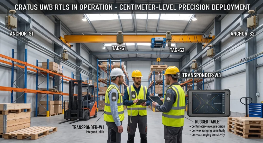
In the landscape of Real-Time Location Systems (RTLS), “close enough” is no longer good enough. Legacy wireless technologies like Wi-Fi and Bluetooth Low Energy (BLE) revolutionized proximity tracking, but their reliance on Received Signal Strength Indicator (RSSI) means their accuracy is inherently bounded to a few meters. In a chaotic industrial environment, a three-meter margin of error is the difference between tracking an asset and losing it completely. RSSI measurements fluctuate unpredictably due to environmental noise, human bodies, and physical obstacles, making true precision impossible.
Enter Ultra-Wideband (UWB). By operating over an expansive RF bandwidth (typically >500 MHz) and transmitting ultra-short, nanosecond-duration pulses, UWB effectively bypasses multipath fading and interference to deliver centimeter-level precision. It doesn’t just verify that a component is in a warehouse; it identifies the exact shelf, bin, and row it occupies. To architect an enterprise-grade UWB RTLS, however, system designers must navigate critical tradeoffs in signaling protocols, node roles, and geometric constraints.
TWR vs. TDoA: The Architectural Showdown
At the heart of any UWB deployment lies the method used to calculate distance. The two dominant approaches are Two-Way Ranging (TWR) and Time Difference of Arrival (TDoA). To understand these mechanisms, we look to foundational industry standards. Decawave—the pioneer behind the ubiquitous DW1000 silicon, later acquired by Qorvo—provided the physical hardware layer that commercialized ultra-precise Time of Flight (ToF) measurements. Meanwhile, software innovators like 7Hugs Labs (also integrated into Qorvo) engineered the advanced software stacks and algorithms necessary to translate raw RF timestamps into ultra-low-latency coordinates.
1. Two-Way Ranging (TWR)
TWR calculates the distance between two devices by measuring the round-trip time of flight of radio packets bouncing between them. An initiating node sends a packet; the responding node receives it and transmits a reply after a deterministic internal delay. The initiator measures the total round-trip time, subtracts the responder’s processing delay, and divides by two to find the exact Time of Flight. Multiplying this by the speed of light yields a highly accurate distance. To mitigate clock drift errors between the two independent crystal oscillators, advanced implementations use Symmetrical Double-Sided TWR (SDS-TWR), which uses a three-message flight exchange to calculate distance with minimal error.
2. Time Difference of Arrival (TDoA)
TDoA functions similarly to an indoor GPS network. Instead of a bidirectional dialogue, signaling is strictly unidirectional. A mobile node emits a single, brief “blink” packet. This packet is intercepted by multiple stationary reference points. Because these stationary points are locked to a master clock network with picosecond-level synchronization, a central location engine compares the difference in arrival times between pairs of receivers. Each time difference defines a hyperbolic curve of possible locations. The intersection of three or more of these hyperbolas reveals the node’s exact 2D or 3D coordinates.
| Metric / Feature | Two-Way Ranging (TWR) | Time Difference of Arrival (TDoA) |
|---|---|---|
| Infrastructure Sync | None required. Anchors operate independently without a shared clock source. | Strictly mandatory. Anchors must be synchronized via high-precision distribution hardware or complex over-the-air wireless protocols. |
| Power Consumption | High. Requires multiple packet transmissions and receptions for every single location update, draining mobile batteries faster. | Ultra-Low. Mobile nodes execute a single, microsecond-long blink packet before returning immediately to a deep-sleep state. |
| Device Density | Limited. Due to heavy airtime consumption per range calculation, network capacity caps out at hundreds of active devices per RF cell. | Massive. Minimal airtime footprint per location fix allows the system to scale to thousands of active devices simultaneously. |
| Deployment Complexity | Low. Easy to install plug-and-play anchors. Minimal upfront site surveying needed. | High. Demands precise anchor placement surveys and continuous monitoring of clock synchronization stability. |
Ideal Use Cases: Choosing Your Approach
The choice between TWR and TDoA is driven by your operational density, infrastructure budget, and asset power constraints.
When TWR is Ideal: Peer-to-Peer Proximity
Ideal for automotive digital key fobs, automated guided vehicles (AGVs) managing ad-hoc collision avoidance, or secure hands-free access control gates. It is also excellent for ad-hoc and temporary deployments, such as construction sites, emergency response zones, or mobile maintenance teams where setting up a highly synchronized, permanently wired anchor grid is physically or financially impractical.
When TDoA is Ideal: High-Density Enterprise Asset Tracking
Best for tracking tens of thousands of manufacturing tools, aerospace components, or personnel across vast industrial complexes. It is essential when tracking small form-factor devices, badges, or low-cost asset tags that must survive for 5 to 7 years on a single CR2032 coin-cell battery.
The Three Tiers of Node Architecture: The CRATUS Paradigm
An enterprise-grade UWB network segments its hardware ecosystem into distinct functional tiers to balance processing power, mobility, and energy availability. CRATUS introduces an updated infrastructure paradigm by redefining how semi-stationary assets are tracked and calculated.
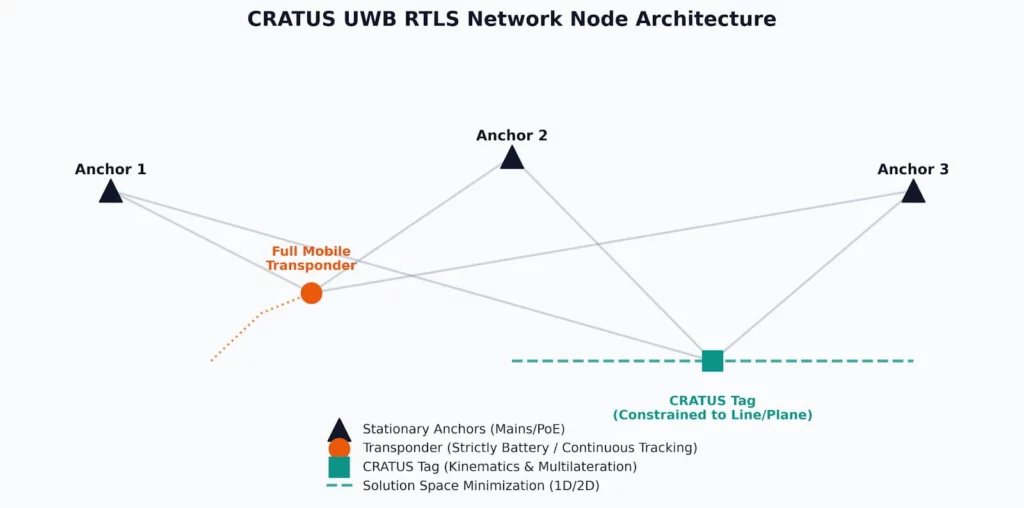
Figure 1: Complete CRATUS UWB RTLS hardware topology, illustrating the relationships between stationary anchors, full mobile transponders, and kinematically constrained tags.
1. Stationary Nodes (Anchors)
Anchors are the rigid structural framework of your spatial coordinates. Mounted permanently at known, survey-verified X, Y, Z positions, anchors act as the receivers or transceivers for the system. Because they must continuously listen for incoming signals, manage network routing, or maintain sub-nanosecond clock alignment, they are always mains-powered or driven via Power over Ethernet (PoE).
2. Full Mobile Nodes (“Transponders”)
Transponders represent highly dynamic elements within the environment—such as active personnel badges or units mounted to fast-moving forklifts. They are strictly battery-powered and require continuous, aggressive tracking with zero lag. To manage this high-throughput requirement without draining the battery in days, transponders leverage advanced software layers (originating from architectures optimized by 7Hugs Labs). They utilize onboard inertial measurement units (IMUs) to put the UWB transceiver into a deep-sleep state when no movement is detected, instantly waking up the moment acceleration is registered.
3. Semi-Mobile / Semi-Stationary Nodes (“Tags”) — The CRATUS Innovation
Bridging the gap are tags, which are deployed on semi-static assets like warehouse inventory pallets, specialized medical crash carts, or shipping containers. Under the CRATUS architectural paradigm, these tags are not assumed to be completely static, nor are they tracked with the brute-force energy footprint of a transponder. Their positions are dynamically changing, but their exact coordinates are resolved using an optimized combination of kinematics and multilateration.
By leveraging kinematic motion models (predicting position based on previous state vectors, velocity trends, and physical acceleration limits), the location engine does not need to compute a raw, multi-anchor location fix from scratch every time. Instead, the mathematical solution space can be heavily constrained. Depending on the asset’s real-world behavior, the solutions can be minimized down to a 2D plane (e.g., assuming a pallet never leaves the floor surface, where Z = constant) or even a 1D line (e.g., tracking automated shelving carts or assembly line carriers locked to fixed tracks). This minimization dramatically reduces the number of required range inputs, cuts power consumption, and eliminates spatial jitter entirely.
Geometric Geographies: Concave vs. Convex Ranging
Even with industry-leading silicon and highly optimized software stacks, the ultimate precision of any RTLS is bound by geometry. This reality is defined by the boundary of your anchor deployment network.
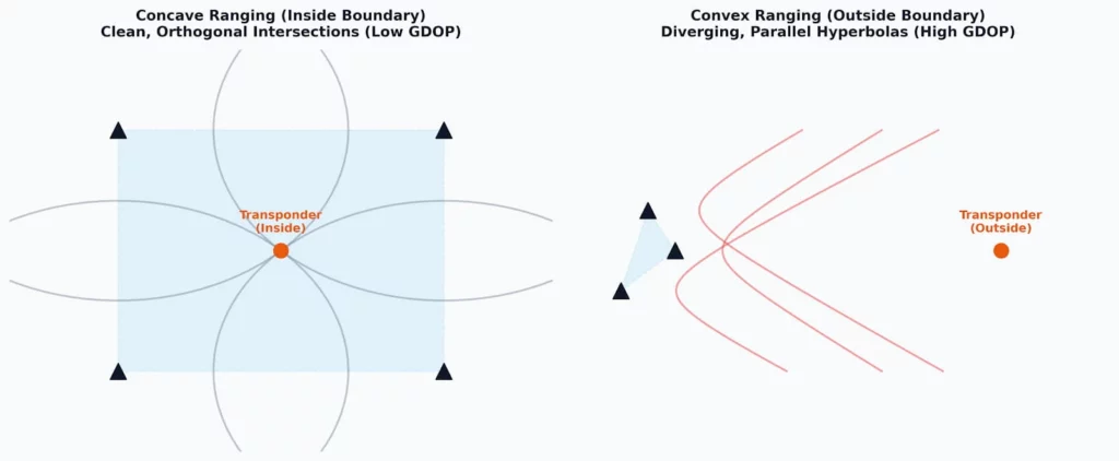
Figure 2: Comparison of Concave ranging (clean orthogonal vector intersections inside the hull) versus Convex ranging (diverging, near-parallel hyperbolic lines outside the hull).
Concave Ranging (Inside the Hull)
Concave ranging occurs when the mobile transponder or tag operates completely inside the three-dimensional volume or perimeter defined by the stationary anchors. In a concave environment, the geometric lines of position (the intersecting circles of TWR or the hyperbolas of TDoA) cross one another at steep, clean, near-orthogonal angles. This yields an exceptionally low Geometric Dilution of Precision (GDOP). Because the geometric lines intersect cleanly, a minor picosecond-level fluctuation in arrival time translates to an imperceptible millimeter-level variation in calculated position.
Convex Ranging (Outside the Boundary)
Convex ranging occurs when a mobile node drifts completely outside the spatial footprint bounded by the anchors. When a transponder exits the perimeter, the mathematical stability of multilateration breaks down due to the extreme sensitivity involved in the multilateration of diverging hyperbolas.
In a TDoA system, your calculated position is derived from the intersection of hyperbola branches. A hyperbola dictates the exact points where the difference in distance to two fixed anchor foci remains constant. As a transponder moves further into a convex region relative to the anchor array, the branches of the tracking hyperbolas begin to flatten out and diverge. Instead of crossing at clean, perpendicular angles, the geometric curves run nearly parallel to each other.
The Physics of the Divergence Penalty
Because the tracking curves are diverging and running nearly parallel in convex space, a microscopic error in the time-of-arrival measurement—whether caused by thermal noise, minor non-line-of-sight (NLoS) body blocking, or antenna group delay—causes the calculated intersection point to slide drastically along the axis of divergence. A tiny timing variance of just 30 picoseconds (which represents a mere 1 cm of physical RF propagation) can shift the calculated coordinate by tens of centimeters or even meters along that parallel path.
To prevent convex tracking degradation, advanced RTLS location engines use Extended Kalman Filters (EKFs) and apply structural constraints (like the CRATUS kinematic plane/line minimization) to weigh down unconstrained convex vectors. Ultimately, however, the primary defense remains structural: deploying anchors strategically to ensure that all critical operational zones remain strictly within a concave geometric layout.

Written by
Founder and CEO, CRATUS Technology, Inc.
Zeki founded CRATUS in 2013 and leads the San Jose team building LiDAR volume measurement systems, IoT sensing platforms, and energy and industrial automation hardware.
Full profileLinkedIn


Interested ?
We would be pleased to send you detailed information about our products or services.
Simply enter your details in the contact form below and we will get in touch with shortly.
CRATUS respects your personal information and keeps it safe. By sending this form, you consent to allow CRATUS to store and process your personal information as stated in our Privacy Policy.